论文链接：High-Resolution Image Synthesis with Latent Diffusion Models

官方实现：CompVis/latent-diffusion、CompVis/stable-diffusion

这一篇文章的内容是 Latent Diffusion Models（LDM），也就是大名鼎鼎的 Stable Diffusion。先前的扩散模型一直面临的比较大的问题是采样空间太大，学习的噪声维度和图像的维度是相同的。当进行高分辨率图像生成时，需要的计算资源会急剧增加，虽然 DDIM 等工作已经对此有所改善，但效果依然有限。Stable Diffusion 的方法非常巧妙，其把扩散过程转换到了低维度的隐空间中，解决了这个问题。

方法介绍

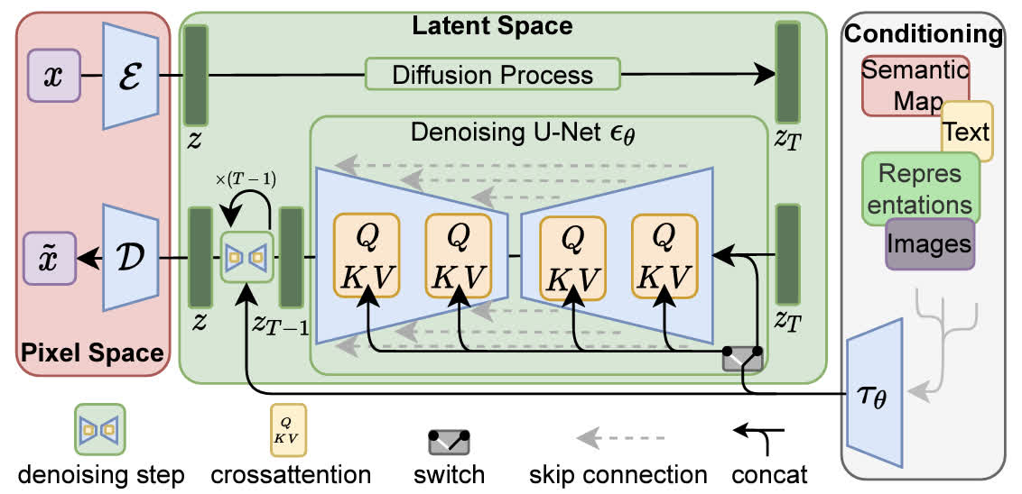
本方法的整体结构如下图所示，主要分为三部分：最左侧的红框对应于感知图像压缩，中间的绿框对应 Latent Diffusion Models，右侧的白框表示生成条件，下面将分别介绍这三个部分。

感知图像压缩

LDM 把图像生成过程从原始的图像像素空间转换到了一个隐空间，具体来说，对于一个维度为 $\mathbf{x}\in {\mathbb{R}}^{H\times W\times 3}$的 RGB 图像，可以使用一个 encoder $\mathcal{E}$将其转换为隐变量 $\mathbf{z}=\mathcal{E}(\mathbf{x})$，也可以用一个 decoder $\mathcal{D}$将其从隐变量转换回像素空间 $\tilde{\mathbf{x}}=\mathcal{D}(\mathcal{E}(\mathbf{x}))$。在转换时会将图像下采样，作者测试了一系列下采样倍数 $f\in \{1,2,4,8,16,32\}$，发现下采样 4-16 倍的时候可以比较好地权衡效率和质量。

在进行图像压缩时，为了防止压缩后的空间是某个高方差的空间，需要进行正则化。作者使用了两种正则化，第一种是 KL-正则化，也就是将隐变量和标准高斯分布使用一个 KL 惩罚项进行正则化；第二种是 VQ-正则化，也就是使用一个 vector quantization 层进行正则化。

Latent Diffusion Models

实际上 latent diffusion models 和普通的扩散模型没有太大区别，只是因为从像素空间变到了隐空间，所以维度降低了。训练的优化目标也没有太大变化，普通的扩散模型优化目标为：
$$L_{\text{DM}}={\mathbb{E}}_{\mathbf{x},ϵ\sim \mathcal{N}(0,1),t}\left[||ϵ-{ϵ}_{\theta }({\mathbf{x}}_t,t)|{|}_2^2\right]$$
而 Latent Diffusion Models 的优化目标只是套了一层 autoencoder：
$$L_{\text{LDM}}={\mathbb{E}}_{\mathcal{E}(\mathbf{x}),ϵ\sim \mathcal{N}(0,1),t}\left[||ϵ-{ϵ}_{\theta }({\mathbf{x}}_t,t)|{|}_2^2\right]$$
在采样时，首先从隐空间随机采样噪声，在去噪后再用 decoder 转换到像素空间即可。

条件生成

为了进行条件生成，需要学习 ${ϵ}_{\theta }({\mathbf{x}}_t,t,y)$，这里使用的方法是在去噪网络中加入 cross attention 层，条件通过交叉注意力注入。在计算注意力时，$\mathbf{z}$为 Query、$y$为 Key 和 Value，具体的内容已经在 Classifier-Free Guidance 的文章中介绍过了，对具体细节感兴趣的读者可以去看一下。

代码解读

Stable Diffusion 有两套主流的代码实现，第一种是 CompVis 的官方实现，第二种是 huggingface 的实现。这里的代码解读都以文生图任务为例。

CompVis 的实现

这个实现的代码比较分散，层次结构不太好梳理，不过可以照着配置文件看各部分都在哪里。这个配置文件有点类似 openmmlab 的那套框架的写法，例如文生图的配置文件 models/ldm/text2img256/config.yaml：

model:target:ldm.models.diffusion.ddpm.LatentDiffusion  params:unet_config:target:ldm.modules.diffusionmodules.openaimodel.UNetModel    first_stage_config:target:ldm.models.autoencoder.VQModelInterface    cond_stage_config:target:ldm.modules.encoders.modules.BERTEmbedder

无关的内容都略去，可以看到顶层的模块是 LatentDiffusion，去噪网络是 UNetModel、encoder 是 VQModelInterface、文本编码器是 BERTEmbedder。

这里主要还是关注 LatentDiffusion的采样过程。具体的采样代码位于 LatentDiffusion.sample：

@torch.no_grad()defsample(self,cond,batch_size=16,return_intermediates=False,x_T=None,verbose=True,timesteps=None,quantize_denoised=False,mask=None,x0=None,shape=None,**kwargs):# 一些数据的封装以及格式转换等等ifshape isNone:shape =(batch_size,self.channels,self.image_size,self.image_size)ifcond isnotNone:ifisinstance(cond,dict):cond ={ key:cond[key][:batch_size]ifnotisinstance(cond[key],list)elselist(map(lambdax:x[:batch_size],cond[key]))forkey incond}else:cond =[c[:batch_size]forc incond]ifisinstance(cond,list)elsecond[:batch_size]# 实际的采样过程returnself.p_sample_loop(cond,shape,return_intermediates=return_intermediates,x_T=x_T,verbose=verbose,timesteps=timesteps,quantize_denoised=quantize_denoised,mask=mask,x0=x0)

可以看到实际的采样过程并不是在这一层进行，这一层只进行了一些封装，例如采样的大小以及条件的数据格式等等，具体的采样则是在 p_sample_loop中进行的：

@torch.no_grad()defp_sample_loop(self,cond,shape,timesteps=None):iterator =tqdm(reversed(range(0,timesteps)),desc='Sampling t',total=timesteps)ifverbose elsereversed(range(0,timesteps))fori initerator:ts =torch.full((b,),i,device=device,dtype=torch.long)img =self.p_sample(img,cond,ts,clip_denoised=self.clip_denoised,quantize_denoised=quantize_denoised)returnimg

去掉一堆杂七杂八的代码之后可以发现在 p_sample_loop中是一个循环，也就对应于一步步进行降噪的过程，具体的降噪在 p_sample中实现：

@torch.no_grad()defp_sample(self,x,c,t,clip_denoised=False,repeat_noise=False,return_codebook_ids=False,quantize_denoised=False,return_x0=False,temperature=1.,noise_dropout=0.,score_corrector=None,corrector_kwargs=None):b,*_,device =*x.shape,x.device    outputs =self.p_mean_variance(x=x,c=c,t=t,clip_denoised=clip_denoised,return_codebook_ids=return_codebook_ids,quantize_denoised=quantize_denoised,return_x0=return_x0,score_corrector=score_corrector,corrector_kwargs=corrector_kwargs)model_mean,_,model_log_variance =outputs    noise =noise_like(x.shape,device,repeat_noise)*temperature    ifnoise_dropout >0.:noise =torch.nn.functional.dropout(noise,p=noise_dropout)# no noise when t == 0nonzero_mask =(1-(t ==0).float()).reshape(b,*((1,)*(len(x.shape)-1)))returnmodel_mean +nonzero_mask *(0.5*model_log_variance).exp()*noise

在 p_sample中，首先用模型预测出了均值和方差（也就是 p_mean_variance，这里就不展开讲了），然后进行了去噪。

综合上述分析来看，如果看原始代码，可能会觉得非常混乱，但是其实去掉不重要的内容之后，核心的代码并不算非常多。这里没有展开具体的 p_mean_variance内部的内容，在 CompVis 的框架中，定义了很多 diffusion 中常用的常量（例如 alphas_cumprod、sqrt_recipm1_alphas_cumprod等）和方法（例如 q_mean_variance、p_mean_variance等），后续我应该还会写一篇文章专门介绍这些内容，这里暂时略过，只需要知道最顶层的 p_mean_variance是预测了均值和方差即可。

huggingface 的实现

相比于 CompVis 的实现，huggingface 的实现更加工程化一点，相关的在 diffusers库中。这个库主要包括三大类元素：models（各种神经网络的实现，unet、vae 等）、schedulers（diffusion 相关的操作，加噪去噪等）、pipelines（high level 封装，相当于 models+schedulers，这个应该是方便用户直接用的）。

这里直接看 diffusers/pipelines/stable_diffusion/pipeline_stable_diffusion.py的采样过程，定义在 __call__函数中：

@torch.no_grad()@replace_example_docstring(EXAMPLE_DOC_STRING)def__call__(self,prompt:Union[str,List[str]]=None,height:Optional[int]=None,width:Optional[int]=None,num_inference_steps:int=50,timesteps:List[int]=None,sigmas:List[float]=None,guidance_scale:float=7.5,negative_prompt:Optional[Union[str,List[str]]]=None,num_images_per_prompt:Optional[int]=1,eta:float=0.0,generator:Optional[Union[torch.Generator,List[torch.Generator]]]=None,latents:Optional[torch.Tensor]=None,prompt_embeds:Optional[torch.Tensor]=None,negative_prompt_embeds:Optional[torch.Tensor]=None,ip_adapter_image:Optional[PipelineImageInput]=None,ip_adapter_image_embeds:Optional[List[torch.Tensor]]=None,output_type:Optional[str]="pil",return_dict:bool=True,cross_attention_kwargs:Optional[Dict[str,Any]]=None,guidance_rescale:float=0.0,clip_skip:Optional[int]=None,callback_on_step_end:Optional[Union[Callable[[int,int,Dict],None],PipelineCallback,MultiPipelineCallbacks]]=None,callback_on_step_end_tensor_inputs:List[str]=["latents"],**kwargs,):

可以看到参数实在是非常的多，我们在这里不关注工程的部分，只关注核心的逻辑。这里的第一个需要关注的点是对生成条件进行编码：

prompt_embeds,negative_prompt_embeds =self.encode_prompt(prompt,device,num_images_per_prompt,self.do_classifier_free_guidance,negative_prompt,prompt_embeds=prompt_embeds,negative_prompt_embeds=negative_prompt_embeds,lora_scale=lora_scale,clip_skip=self.clip_skip,)# For classifier free guidance, we need to do two forward passes.# Here we concatenate the unconditional and text embeddings into a single batch# to avoid doing two forward passesifself.do_classifier_free_guidance:prompt_embeds =torch.cat([negative_prompt_embeds,prompt_embeds])

这里实际上还有 LoRA 和 IP-Adaptor 相关的处理，暂时省略。可以看到这里对生成的 prompt 进行了编码，并且不仅有正常的 prompt，还有 negative 的 prompt，这是为了做 classifier-free guidance。并且由于两个 prompt 需要分别推理，这里还将其在 batch 维度拼接，来进行并行化。随后获取 timesteps：

timesteps,num_inference_steps =retrieve_timesteps(self.scheduler,num_inference_steps,device,timesteps,sigmas)

然后初始化噪声，这个就相当于 ${\mathbf{x}}_T$：

num_channels_latents =self.unet.config.in_channelslatents =self.prepare_latents(batch_size *num_images_per_prompt,num_channels_latents,height,width,prompt_embeds.dtype,device,generator,latents,)

上边准备了 $\mathbf{x}$、timestep 以及 condition，现在就可以正式进行生成了：

num_warmup_steps =len(timesteps)-num_inference_steps *self.scheduler.orderself._num_timesteps =len(timesteps)withself.progress_bar(total=num_inference_steps)asprogress_bar:fori,t inenumerate(timesteps):# expand the latents if we are doing classifier free guidancelatent_model_input =torch.cat([latents]*2)ifself.do_classifier_free_guidance elselatents        latent_model_input =self.scheduler.scale_model_input(latent_model_input,t)# predict the noise residualnoise_pred =self.unet(latent_model_input,t,encoder_hidden_states=prompt_embeds,timestep_cond=timestep_cond,cross_attention_kwargs=self.cross_attention_kwargs,added_cond_kwargs=added_cond_kwargs,return_dict=False,)[0]# perform guidanceifself.do_classifier_free_guidance:noise_pred_uncond,noise_pred_text =noise_pred.chunk(2)noise_pred =noise_pred_uncond +self.guidance_scale *(noise_pred_text -noise_pred_uncond)ifself.do_classifier_free_guidance andself.guidance_rescale >0.0:# Based on 3.4. in https://arxiv.org/pdf/2305.08891.pdfnoise_pred =rescale_noise_cfg(noise_pred,noise_pred_text,guidance_rescale=self.guidance_rescale)# compute the previous noisy sample x_t -> x_t-1latents =self.scheduler.step(noise_pred,t,latents,**extra_step_kwargs,return_dict=False)[0]

可以看到有一些为了 classifier-free guidance 进行的处理，其他的都是正常 diffusion 的操作。最后将隐变量解码回像素空间得到生成结果：

image =self.vae.decode(latents /self.vae.config.scaling_factor,return_dict=False,generator=generator)[0]

总结

最近看了这么多文章，感觉比较成功的 researcher 的工作都是连贯的。就像宋飏研究 sliced score matching，然后紧随其后做出了 score-based generative model；又如 OpenAI 训出 CLIP 然后基于 CLIP 做了一系列文生图的工作。今天这篇文章看起来也是 CompVis 把 VQGAN 迁移到 diffusion models 上的成果，感觉对平时做研究的启发还是很大的，我个人一直以来研究方向都比较摇摆不定，也应该反思学习一下。

参考资料：

1. diffusion model(五)：LDM: 在隐空间用diffusion model合成高质量图片
2. 扩散模型（六）| Stable Diffusion

本文原文以 CC BY-NC-SA 4.0 许可协议发布于 笔记｜扩散模型（七）：Latent Diffusion Models（Stable Diffusion）理论与实现，转载请注明出处。